Best practices: Getting your code working in the Large Scale

Author: Federico Pedron (BSC)

Going from a few hundred cores to tens of thousands presents several challenges that might not even be related to the software itself. Rather, they are often due to how a given code is being run on the machine. In this guide, we will present several options that do not involve reworking the code you are using, but that might allow you to achieve the best scalability possible and solve hard-to-track errors.

Most of these recommendations (presented in Sections 1 and 2) will be focused on MareNostrum 5, but the majority of the tricks presented here can be easily translated to other HPC centres. Section 3 will present a sample application of the topics covered herein, while the last section of this guide (Section 4) will cover a few options to analyze and debug codes at a large scale.

It is worth noting that there is a lot of trial-and-error involved in finding the correct or optimal settings for your runs. No set-up will be equally effective for all codes, or even all inputs for similar codes. But there is a lot to gain by spending a few minutes testing different configurations.

Without further ado, let’s begin with the most important aspect for large scale simulations: CPU affinity.

1 – Improving CPU affinity

CPU affinity is usually a critical component in ensuring optimal HPC performance. It is, by far, the most significant aspect in terms of performance. By affinity, we usually mean two distinct but complementary features: how each MPI task is placed on the physical cores (binding) and how these tasks are distributed across the cores (distribution or placement).

1.1 – Core binding

MPI implementations provide roughly the same options regarding binding; however, the options are slightly different between srun, and mpirun or mpiexec. Take the following example, in which we bind the tasks to cores:

mpirun --bind-to cores [arguments]
srun --cpu-bind=cores [arguments]

This type of binding means that once the task starts using a given core, it will not leave that core until it finishes. Other types of bindings (such as hwthreads, or sockets) may allow the tasks to jump between cores, but within a given boundary (NUMA node, socket, node).

Depending on how MPI or SLURM is configured within your machine, there might be some type binding happening by default. In the case of MareNostrum 5, it is necessary to disable SLURM binding when using mpirun; this is because mpirun uses srun underneath, which itself forces certain bindings. Therefore, to prevent issues, it is mandatory to set the environment variable SLURM_CPU_BIND=none when using mpirun:

export SLURM_CPU_BIND=none
mpirun --bind-to cores [arguments]

1.2 – Core placement

Note: Some programs, in particular modern python workflows, attempt to handle core placement by themselves. In these cases, most of the information here will not affect your performance.

The second aspect of CPU affinity is the core placement, by which each task gets assigned each physical core. Both srun and mpirun provide several clever ways to place the tasks onto cores. The most common ones are by processing elements (PE), or by explicit CPU mapping (i.e. specify the exact cores’ IDs used in each node).

# mpirun variants
mpirun --map-by core:PE=36 [arguments] # Number of processing elements per task, in this case, 36 cores per task
mpirun --cpu-set=0,27,56,83 [arguments] # Use cores 0, 27, 56 and 83 from each node.

# srun variants
srun --distribution=block:cyclic  [arguments] # Follow a block cyclic distribution, similar to PE for mpirun.
srun --cpu-bind=map_cpu:0,27,56,83  [arguments] # Use cores 0, 27, 56 and 83 from each node

In the following paragraphs there will be several concrete examples of these, applied to MareNostrum 5 in particular. It is strongly suggested to take a look at the SLURM documentation and the OpenMPI documentation for further options, since there are several ways to apply the CPU mapping.

Getting an optimal core placement requires knowledge of the specific hardware you are running on. Fortunately, EuroHPC centres provide documentation on the hardware specifics for each node. Here are a few examples of these:

• MareNostrum 5: GPP, ACC
• Leonardo: Booster and DCGP
• LUMI: LUMI-C, LUMI-G
• MeluXina: CPU and GPUs
• Karolina: CPUs and GPUs
• VEGA: CPU , GPU 
• Discoverer: Discoverer CPU, Discoverer+ GPU 
• Deucalion: CPUs and GPUs

Core placement becomes especially relevant when running hybrid MPI-OpenMP and/or MPI-GPU applications. In the case of MPI-OpenMP applications, placements can be cleverly assigned so that all threads spawned by a task fall all on the same socket, thus preventing performance issues with OpenMP.

Take for example MareNostrum 5 GPP, which has nodes with 112 cores distributed across two NUMA domains:

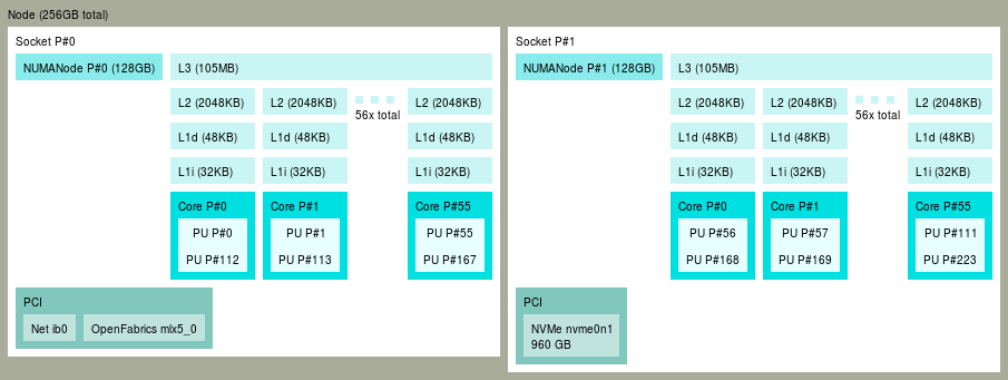
Now, consider a job that requires 4 tasks per node, using 28 cores each (28 x 4 = 112):

# mpirun variants
mpirun --map-by core:PE=28 [arguments]

# srun variants
srun --distribution=block:block [arguments]

In this way, we ensure that each task gets 28 consecutive cores: task 1 gets 0-27, task 2 gets 28-55, task 3 gets 56-83, and task 4 gets cores 84-111. Subsequent tasks repeat this pattern; for example, task 5 gets the same core IDs as task 1 (in a different node). This ensures that all OpenMP threads will always be spawned within the same NUMA node, preventing slowdowns due to an inefficient OpenMP distribution.

If this distribution is not explicitly set, some default will be set. For srun, this default will use the block:cyclic distribution: this means it will be first filling each node, and within each node it will be alternating tasks in the sockets. In the example above, this means task 1 gets 0-27, task 2 gets 56-83, task 3 gets 28-55, and task 4 gets cores 84-111 (note the exchange between tasks 2 and 3).  For mpirun the default handling is not straightforward: it will depend on each MPI implementation (IntelMPI, OpenMPI, NVHPCX) and how it is configured in each machine.

With hybrid CPU-GPU implementations, a similar rationale applies. In an HPC node, usually  not all GPUs are equally close to all NUMA nodes. Take, for example, the node architecture of MareNostrum 5 ACC:

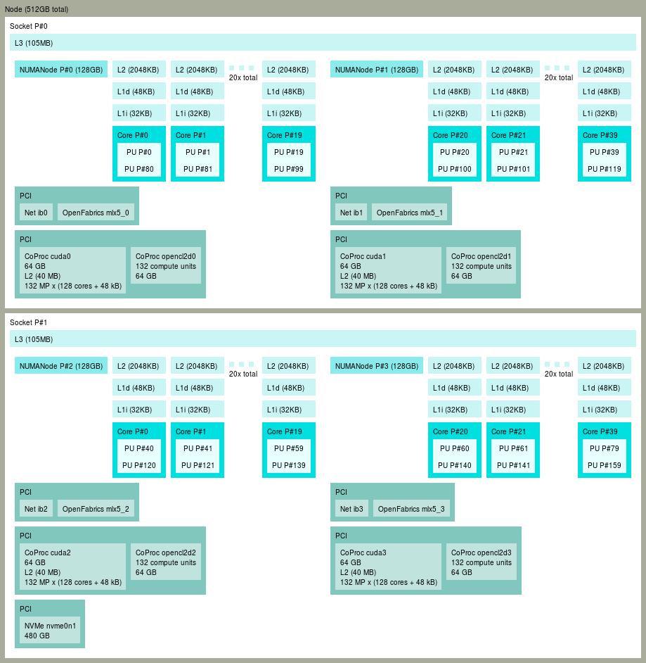
You can see here that not only GPUs (CoProc Cuda X) are distributed across different sockets, but also that each GPU is attached to a given NUMA node. In terms of cores-to-GPUs preference, this means that cores 0–19 should use GPU 0, cores 20–39 should use GPU 1, cores 40–59 should use GPU 2, and cores 60–79 should use GPU 3.

For NVIDIA GPUs, this is usually handled by the environment variable CUDA_VISIBLE_DEVICES; for AMD GPUs you should rely on the analogous ROCR_VISIBLE_DEVICES. Other variables exist for specific applications, such as HIP_VISIBLE_DEVICES, but the first two cover most of the needs for EuroHPC machines.

With this information, you can create a wrapper for your code that both a) binds cores to tasks, and b) ensures that cores are bound to the closest GPU available. A sample wrapper for MareNostrum 5 ACC could be this one:

CODE SNIPPET

Then, this wrapper can be called under MPI, just before launching the program:

srun [options] wrapper.sh program.exe [program_options]
mpirun --bind-to none [options] gpu_wrapper program.exe [program_options]

In the case of MareNostrum 5, a more complete wrapper is provided in the shape of bsc_affinity; however, different HPC centres handle this differently. You can use bsc_affinity as you would use any other wrapper:

module load bsc
export SLURM_CPU_BIND=none

# For OpenMPI+CUDA, srun
srun [options] bsc_affinity program.exe [program_options]

# For NVHPCX, mpirun
mpirun --bind-to none [options] bsc_affinity program.exe [program_options]

1.3 – Getting hardware topology information

In cases where no documentation is available, there are a few ways to get hardware topology information for any given machine. Remember that login nodes can be slightly different from compute nodes, so the better option is to send a job (or allocation) to a compute node before starting.

The most commonly found tool to get hardware information (available on all HPC centers) is hwloc. In particular, this information can be acquired from hwloc-ls (or lstopo, which is equivalent):

$ hwloc-ls
Machine (503GB total)
  Package L#0 + L3 L#0 (105MB)
    Group0 L#0
      NUMANode L#0 (P#0 126GB)
      L2 L#0 (2048KB) + L1d L#0 (48KB) + L1i L#0 (32KB) + Core L#0
        PU L#0 (P#0)
        PU L#1 (P#80)
      L2 L#1 (2048KB) + L1d L#1 (48KB) + L1i L#1 (32KB) + Core L#1
        PU L#2 (P#1)
        PU L#3 (P#81)
      L2 L#2 (2048KB) + L1d L#2 (48KB) + L1i L#2 (32KB) + Core L#2
        PU L#4 (P#2)
        PU L#5 (P#82)

You will find a lot of information in the output, which might be hard to parse.  However, this output can be better understood by trimming some of the information, using hwloc-ls --no-smt --ignore Net --merge --no-bridges:

$ hwloc-ls --no-smt --ignore Net --merge --no-bridges

Machine (503GB total)
  Package L#0
    Group0 L#0
      NUMANode L#0 (P#0 126GB)
      Core L#0
      Core L#1
      ...
      Core L#18
      Core L#19
      PCI 00:17.0 (SATA)
      PCI 01:00.0 (Ethernet)
        Net "enp1s0"
      PCI 03:00.0 (VGA)
      PCI 18:00.0 (InfiniBand)
        Net "ib0"
        OpenFabrics "mlx5_0"
      PCI 1b:00.0 (3D)
      PCI 6b:00.0 (Co-Processor)
      PCI 6d:00.0 (Co-Processor)

With this information, we can see how many cores (“Core L#”) are under each NUMA node (“NUMANode L#”), and their indexes. This is very useful information to keep in mind for hybrid OpenMP+MPI applications. We also get information about the infiniband connectors and how they relate to each NUMA node (“mlx5_”).

However, while the output also shows the GPUs (“Co-Processor”), it still misses vital information. In particular, we do not know whether the GPUs themselves are connected via special connectors (NVLink), nor can we identify which physical GPU corresponds to a given GPU ID (such as the one used for CUDA_VISIBLE_DEVICES). For this kind of information, we need vendor-provided tools, that are also available in all HPC centres. On MareNostrum 5, we rely on nvidia-smi topo -m, which show the connection matrix between all accelerators:

               GPU0            GPU1           GPU2           GPU3           NIC0           NIC1           NIC2           NIC3           NIC4           NIC5           CPU Affinity      NUMA
GPU0            X              NV6            NV6            NV6            PXB            SYS            SYS            SYS            SYS            SYS            0-19,80-99        0
GPU1            NV6            X              NV6            NV6            SYS            PXB            NODE           NODE           SYS            SYS            20-39,100-119     1
GPU2            NV6            NV6            X              NV6            SYS            SYS            SYS            SYS            PXB            SYS            40-59,120-139     2
GPU3            NV6            NV6            NV6            X              SYS            SYS            SYS            SYS            SYS            PXB            60-79,140-159     3

In this matrix, GPUX indicates each GPU index, and NICX corresponds to all network connectors (InfiniBand). More importantly, NUMA Affinity and CPU Affinity show us which CPUs are physically closer to each GPU, which allows us to create wrappers in the style of the ones presented in the previous section.  For example, take the GPU0 line: it is connected to all other GPUs via NVLink (NV6), and at the end of the table we see that it has better affinity with NUMA node 0. We also see that the closest network device is NIC0 (mlx5_0), by virtue of it being connected via PXB (fast PCI bridges) and not SYS (which needs to traverse NUMA nodes).

If you go back to our original wrapper, you will see that the core assignments and network device assignment follow exactly the information presented in that table:

0)
    export CUDA_VISIBLE_DEVICES=0
    export mycores="0-19"
    export UCX_NET_DEVICES=mlx5_0:1
;;
...
3)
    export CUDA_VISIBLE_DEVICES=3
    export mycores="60-79"
    export UCX_NET_DEVICES=mlx5_5:1
;;

See how CUDA_VISIBLE_DEVICES=3, for example, goes along cores “60-79” and the network device mlx5_5.

Note: For AMD GPUs, the analogous rocm-smi (or amd-smi) is available.  rocm-smi --showtoponuma produces information similar to nvidia-smi topo -m.

1.4 – Testing binding and core placement

The very first thing to test when trying to set bindings and placement is that the directives you are using produce the expected result. This can easily be tested using simple commands or bash scripts.

For example, doing cat/proc/self/status on any GNU/Linux system will give us all of the information regarding a process. So if we run:

srun -n 1 -c 1  grep Cpus_allowed_list /proc/self/status

bash
Cpus_allowed_list:     0

bash
Cpus_allowed_list:     0,112

Notice the double numeration. Since hyperthreading is enabled, you are seeing two indexes per CPU: one what goes from 0 to N-1, and another that goes from N to 2N-1 (with N being the total number of cores per node), corresponding to each of the processing units per CPU.

Note: Hyperthreading is usually undesirable at the large scale (and most HPC in general). In order ensure that hyperthreading is disabled, you can set the SBATCH options --threads-per-core 2 and/or --hint nomultithread, depending on the machine.

This can also be used to check how OpenMP threads are being assigned. For example:

$ srun -n 2 -c 4 grep Cpus_allowed_list /proc/self/status
Cpus_allowed_list:     56-59
Cpus_allowed_list:     0-3

You can see here that each of the two tasks has 4 CPUs assigned, with one using cores 0 through 3 and the other one using cores 56 through 59.

Moving now onto GPUs: if you want to check whether your GPU wrapper is doing the placement correctly, you can instead do a simple bash script that joins the result of the above commands with the GPU indexing variable (CUDA_VISIBLE_DEVICES or ROCR_VISIBLE_DEVICES). For completeness, we can also add the task ID. For example:

CODE SNIPPET

We can then run this script under any custom wrapper:

$ srun -n 4 -c 20 gpu_wrapper ./check_cpu_placements
Task 0 - CPUs allowed:   0-19 - GPUs allowed: 0
Task 1 - CPUs allowed: 20-39 - GPUs allowed: 1
Task 2 - CPUs allowed: 40-59 - GPUs allowed: 2
Task 3 - CPUs allowed: 60-79 - GPUs allowed: 3

2 – HPC Toolbox: UCX, MPI Collectives, I/O and NVIDIA MPS

In this section, we will cover a few tricks and tools that are not necessarily a primary concern for all cases. However, in the specific codes or workflows where they matter, these will impact performance significantly. They can even enable running at a scale that was not previously reachable with other options.

2.1 – Setting UCX options

UCX (Unified Communication X) is the middleware that interfaces between the MPI functions (coming from OpenMPI, NVHPCX, IntelMPI, and others) and the hardware involved in the inter-process communications. There are other similar interfaces, such as OFI (the OpenFabrics Interface); however, UCX is present in almost all EuroHPC centres and has been proved very reliable in general (One exception is LUMI, which does not support UCX at all. OFI with the CXI provider is the only option for high-speed communication, so the following pieces of advice will not apply to it).

Default UCX options are usually good enough, hence why UCX is generally transparent to the user and barely ever mentioned. However, getting acquainted with it is important to move into the large-scale scene. For example, spurious communication errors may appear if UCX internal heuristics fail to select an appropriate transport layer. These are the kinds of errors that rarely appear when using a few nodes but become increasingly prevalent when moving into hundreds of nodes with thousands of tasks.

Usually, just ensuring a UCX library is loaded in the environment and that the MPI libraries have been compiled with UCX support is enough to handle most of these errors. On MareNostrum 5 all MPI implementations support UCX, and specific UCX modules may be loaded via:

module load ucx

Be sure to check the different modules available with module avail ucx. Once the module is loaded, you can fine tune several UCX functionalities with environment variables. Out of the plethora of options available, fortunately only one is relevant: UCX_TLS (Transport Layer Selection). This environment variable allows us to select different protocols for communication between tasks. Take for example:

export UCX_TLS=self,sm,dc_mlx5

In this example we choose the options “self” (loopback for the process to communicate with itself), “sm” (all shared memory) for intra-node communication, and “dc_mlx5” (dynamic communication accelerated via InfiniBand) for communication between nodes. There are several options available for the latter two:

• Intra-node communication: sm (selects all, lets UCX decide), sysv, posix, cma, knem, xpmem.
• Inter-node communication: dc_mlx5, rc_mlx5, ud_mlx5 (note: the _x suffix is synonymous with _mlx5).
• Accelerators: cuda, rocm.

Typically, rc_mlx5 is the best performing option, but it will crash when executing a large number of tasks due to saturation of the network device memory. If your program requires a lot of tasks per node, you want to use dc_mlx5; however, UCX default internals may sometimes erroneously choose rc_mlx5, and then crash due to insufficient network device memory.

In case you want to check out which options are available for UCX_TLS, you can always run ucx_info -d. The output of this command can be quite daunting, but you can filter out the relevant information with something like the following:

ucx_info -d | grep "Transport" -A2

This produces an output similar to the one below, in which you can see not only the name of the transport, but also the type of transport and the associated devices (if any):

#      Transport: ud_mlx5
#         Device: mlx5_5:1
#           Type: network
--
#      Transport: knem
#         Device: memory
#           Type: intra-node
--
#      Transport: xpmem
#         Device: memory
#           Type: intra-node

It is generally advisable to pick at least one transport from each category (network, intra-node, loopback). If you have accelerators present, watch out for the “accelerator” category, and see if there are any other relevant intranode options (such as cuda_ipc, for example).

If UCX_TLS is not set at all, UCX will rely on internal heuristics to set the appropriate transport layer. If multiple options are present for the same type on transport (for example, UCX_TLS=posix,sysv), UCX will try to pick the appropriate one from the ones explicitly set in UCX_TLS.

2.2 – MPI Implementations, MPI and UCX versions

It is often the case that some performance gains can be achieved by changing the underlying MPI implementation, the version of said implementation, or even the version of UCX employed.

It is usually a good idea to test the different versions available on the machine for both MPI (no matter if it is IntelMPI, OpenMPI, NVHPCX, CrayMPI, or any other) and UCX.

To get an example of how widely different the performance may be across these, you can have a look at the BSC report on OSU microbenchmarks. While UCX versions were not part of the testing, MPI implementations were. While of course there are differences between OpenMPI and IntelMPI, it is also interesting to find the differences between OpenMPI 4 and OpenMPI 5 (for example, different results can be seen for MPI_Broadcast latency). While the report is exhaustive, the take-home message here is that testing the different versions of the MPI implementations available is often worth the time and effort.

Finally, testing versions of MPI implementations is not only a matter of performance: some applications might, for example, experience memory leaks with specific versions of IntelMPI.

2.3 – MPI Collectives

All MPI implementations support different algorithms for MPI collectives. Usually, the algorithm used depends on internal heuristics for that implementation, but there are ways to force a specific algorithm for a given run. If the code used relies heavily on a specific MPI collective, it might be worth trying a few different variants to see how they affect performance.

For IntelMPI, the family of variables are called I_MPI_ADJUST_{COLLECTIVENAME}, where COLLECTIVENAME is any of AlltoAll, AllGather, Bcast, etc. . This environment variable is set to an integer number representing the index of each algorithm, which can be referenced in the IntelMPI documentation. Take for example:

# Set the "Ring" algorithm for AllGatherV.
export I_MPI_ADJUST_ALLGATHERV=3

In the case of OpenMPI and related implementations (like NVHPCX), the algorithm is set via the “–mca coll_tuned” family of variables, which can be found in the OpenMPI documentation. For example:

# Set the "Modified Bruck" algorithm to AlltoAll.
mpirun --mca coll_tuned_use_dynamic_rules 1 --mca coll_tuned_alltoall_algorithm 3 [...]

2.4 – MPI I/O

Most HPC codes implement MPI I/O in some capacity, usually via pNetCDF. When MPI I/O is used for input/output, the default I/O component (ompio) is usually less performant (and less stable) than the alternatives. On MareNostrum 5, it is always recommended to use romio instead, which can be set via:

export OMPI_MCA_io=romio321

Some implementations, such as IntelMPI, use romio by default. If MPI I/O is a dominant part of your code, ask the HPC centre of choice whether they have any recommendations on this regard.

2.5 – Using NVIDIA MPS

For some hybrid CPU-GPU codes, there are cases in which multiple MPI tasks can use the same GPU concurrently. To avoid interference and bottlenecks, NVIDIA provides the Multi-Process Service (MPS), which enforces a designated space for each task within the GPU. This greatly increases GPU utilization, especially in those cases where multiple smaller tasks are running on the same NVIDIA GPU.

Using NVIDIA MPS usually involves wrapping the code to start and stop the MPS service before and after running. The service needs to be started once per node, so only one task for each node needs to activate and deactivate it. You can, for example, rely on the environment variable SLURM_LOCALID for this purpose:

CODE SNIPPET

With the wrapper above, you can just run:

srun [options] mps_wrapper [other_wrapping_scripts] program [program_options]

In the case of MareNostrum 5, NVIDIA MPS is ready to use, and a wrapper is already provided:v

module load mps

# For srun
srun [options] mps [wrapping_script] program [program_options]

# For mpirun
mpirun --bind-to none [options] mps [wrapping_script] program [program_options]

3 – Let’s put it into practice!

It’s time to put some of the concepts we have explored above to the test. We will use a very simple MPI SENDRECEIVE program written in C; in this example, each task has a “peer” to communicate with. These peers are chosen according to the total number of tasks: if the total amount of tasks is N, then the peer for task a (with a < N/2) is b = N/2 + a. This means that the first half of the tasks is communicating with the second half exclusively. You can find this piece of code here:

CODE SNIPPET

All results correspond to the MareNostrum 5 – General Purpose Partition (MN5-GPP), which has CPU-only nodes of 112 cores each. All calculations have been done on 16 nodes . First we test the most relevant part of the setup, the core placement, with the code provided. Then we proceed to test different MPI implementations, and UCX options.

3.1 – Testing core placement

We start by testing core placement using the default modules available in MareNostrum 5 GPP: Intel compilers 2023.2, IntelMPI 2021.10 and UCX 1.15.0. We test four combinations of task distribution, using SLURMS’s distribution option as mentioned before: block:block, block:cyclic, cyclic:block, and cyclic:cyclic.

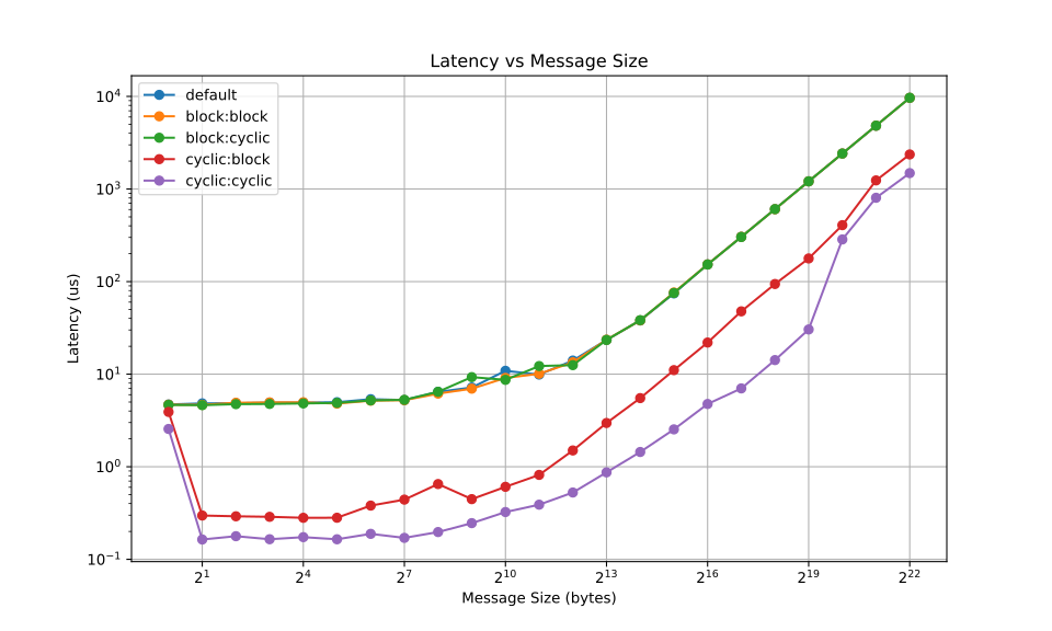
As we can see, the cyclic:cyclic distribution provides the optimal core placement for tasks. This might seem obvious from the type of communications performed, but scientific pieces of software are usually much more complex than this simple test. Thus, optimal placement will not always be straightforward: it will often be a combination of the number of threads per task, and the types of communications that are limiting performance.

3.2 – Testing MPI implementations

We now test different MPI implementations: two versions of IntelMPI, and two versions of OpenMPI. The first, IntelMPI 2021.10, corresponds to the default modules available in MareNostrum 5.

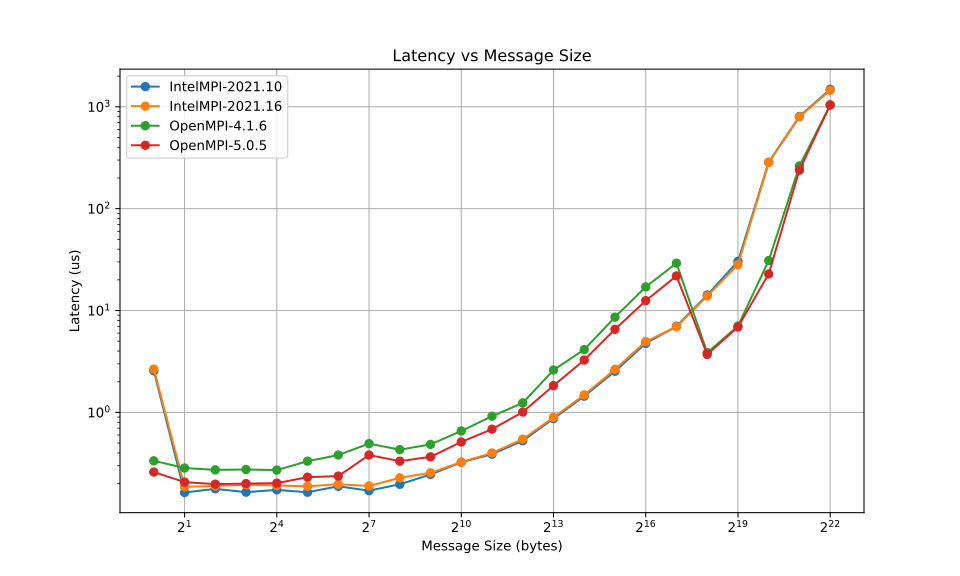
We can see that no implementation is better than the other one: both IntelMPI implementations are similar and perform best for short- to mid-sized messages; whereas, both OpenMPI implementations work best for large messages. For this example, we will stick to the default IntelMPI version (2021.10). In addition, since this is a simple SEND_RECEIVE, there is no MPI collective tuning available, so there is no need to tune MPI environment variables in general.

If we are using a program that has consistent message sizes across all codes, then it could be possible to predict the best implementation to be used from Figure 2. However, scientific software tends to have widely different MPI functions and message sizes, so it quickly becomes very hard to predict. Thus, as with core distribution, it becomes necessary to test available implementations with sample inputs before moving on to full production runs. As shown in Figure 2, it is evident that choosing the right implementation provides a non-negligible speed up, with one implementation communicating twice as fast as another one in some cases.

3.3 – Testing UCX options

Now that we have tested core placement and MPI implementations, it might be worth exploring whether UCX impacts the speed of our computations. Using IntelMPI 2021.10 with a cyclic:cyclic distribution, we make two different tests for UCX_TLS: one for intra-node communications (testing the posix, sysv and knem transport layers) and another one for the inter-node communications (testing dc_mlx5, rc_mlx5 and rc_verbs). In both cases, we compare to the default scenario of not declaring any TLS and letting UCX decide by itself.

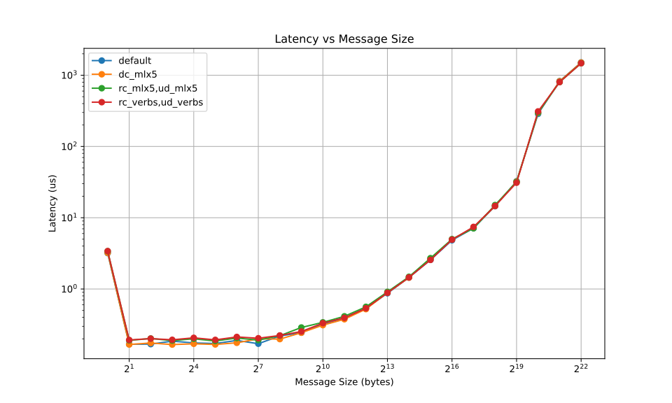
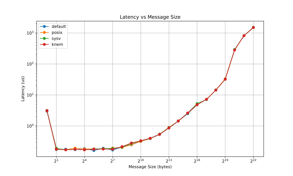
For this piece of code, there is very little difference between UCX_TLS options, and leaving the default is probably the best option. This also holds for different UCX versions (we tested UCX 1.16 and UCX 1.17, not pictured here to avoid redundancy). However, differences arise if we use the non-optimal distribution “block:cyclic” instead:

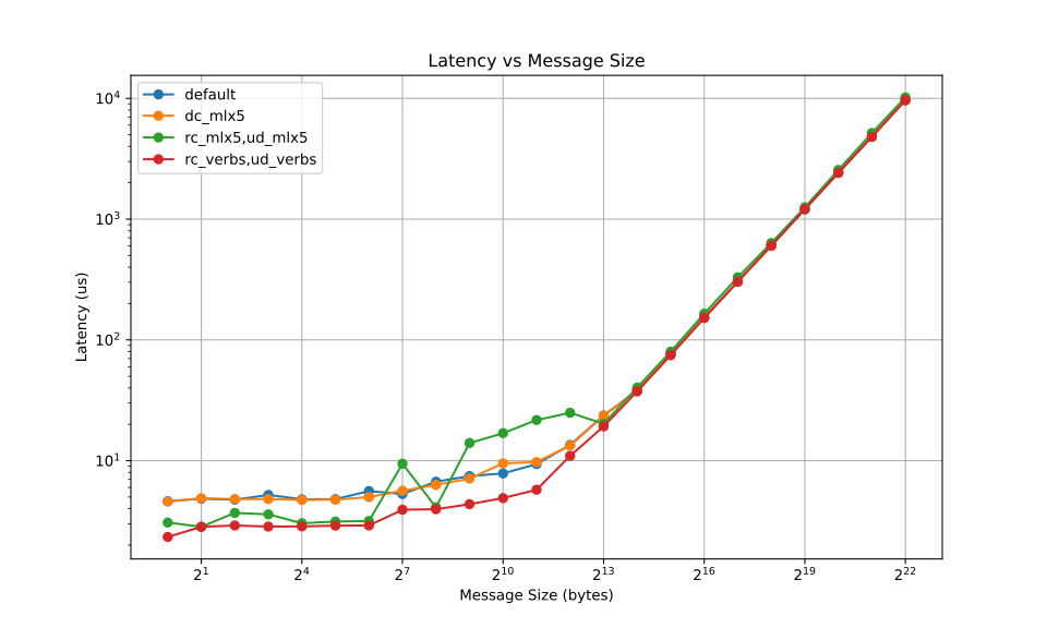
It becomes clear in this scenario that choosing the rc_verbs TLS is the best option. Given that choosing the appropriate distribution still yields the highest benefits, much more so than changing UCX_TLS, this is not a realistic scenario. However, it is useful to illustrate that experimenting with different UCX_TLS options might be worth the time spent.

4 – Debugging and profiling your code at a large scale

4.1 – Debuggers

Debugging at a large scale can be quite challenging, since most of the commonly used debugging tools (such as GDB or Valgrind) were not originally intended for large multi-node systems. On MareNostrum 5, Linaro DDT is also available, providing an easier way to analyze multi-process jobs. However, due to the license provided, DDT is limited to 4000 MPI tasks maximum. Other proprietary debuggers might be available at other centers.

We will focus here on GDB instead, which is readily available on all machines.

Note: To get source code information from the debugger (i.e. debugging symbols), your program needs to be compiled with the -g option. When using CUDA, nvcc -G also ensures that debugging information is provided for devices (i.e. in the GPU).

4.1.1 – Using GDB at the large scale

GDB usage on large-scale jobs is a bit tricky and might depend on the issue you are trying to tackle. If, for example, the program you want to debug is crashing due to a segmentation fault (or similar), then you can just run a gdb script using gdb -x:

echo “run
bt
exit” > gdbscript

mpirun gdb -x gdbscript --args PATH-TO-PROGRAM/program [program options]

This will execute the program under gdb and run a backtrace (bt) once it’s done.

Other times, something completely different might be happening: for example,  it may be that the program gets stuck in a specific communication or loop. In these cases, it is useful to attach to each process of the same run under each node and get the stack trace for all processes. This can be done using a script like this one:

CODE SNIPPET

This script will generate the stack trace for all processes that are currently running across all nodes for a given job.

4.2 – Profiling

Note: The information contained in this section is specific to MareNostrum 5. Each HPC center may offer different tools for profiling, depending on their specific software stack and hardware configuration. However, some of the concepts presented here can be transferred to other profilers.

MareNostrum 5 offers several ways to profile your code and gain insights on potential bottlenecks your calculations might be facing. All tools presented herein might be available in other HPC centers, but if not, they are fairly straightforward to install.

A fair warning when generating traces with Extrae, HPC toolkit, or any other profiler: trace files can easily become huge for large numbers of tasks, going rapidly into the terabyte scale if you are not careful.

4.2.1 – TALP

TALP is available on the cluster, and while the scope of the library might be limited, it gives you many global insights essentially for free in terms of computational effort.

TALP is part of the DLB suite and works by preloading the appropriate MPI library. In MareNostrum 5, you can do this in the following fashion:

#SBATCH --constraint=perfparanoid

module load dlb

export LD_PRELOAD=”$DLB_HOME/lib/libdlb_mpi.so”

srun [arguments]

The preloaded library is independent of whether you are using mpirun or srun, but it is important to choose the appropriate one for the MPI implementation you are using (IntelMPI, OpenMPI, etc.). When loading the dlb module on MareNostrum, the module itself tries to get a good initial guess by taking a look at the modules that are already loaded. If this detection fails, it will default to the GCC-OpenMPI variant.

When using TALP, you will find a summary like this one at the end of your output:

DLB[:]: ######### Monitoring Region App Summary #########
DLB[:]: ### Name:                       MPI Execution
DLB[:]: ### Elapsed Time :              12.87 s
DLB[:]: ### Parallel efficiency :       0.70
DLB[:]: ###   - Communication eff. :    0.91
DLB[:]: ###   - Load Balance :          0.77
DLB[:]: ###       - LB_in :             0.79
DLB[:]: ###       - LB_out:             0.98

Further information might be obtained depending on a few environment variables, but they will always reflect information for the entire run. We suggest taking a look at the TALP documentation to get further options.

4.2.2 – Extrae/Paraver

MareNostrum 5 offers support for traces generated by the Extrae tool, which can be read by Paraver. Using Extrae also requires LD_PRELOAD, and can be used by setting the following options:

#SBATCH --constraint=perfparanoid

module load extrae

export EXTRAE_CONFIG_FILE=./extrae.xml
export LD_PRELOAD=${EXTRAE_HOME}/lib/libmpitrace.so

The extrae.xml file contains all required options for  Extrae. In $EXTRAE_HOME/share/example, there are various examples for different use cases, but probably the most relevant option (in terms of data generated) is burst mode:

<trace enabled="yes"  
 initial-mode="burst"
 type="paraver"
>

  <burst enabled="yes">
    <!-- Threshold in microseconds -->
    <threshold enabled="yes">10000u</threshold>

    <!-- Report MPI statistics? -->
    <mpi-statistics enabled="yes" />
  </burst>

You can lower the burst threshold to increase the sampling, but doing so will greatly increase the size of the traces.

The traces generated in Extrae can later be explored with Paraver, which is also available on the machine:

module load paraver

wxparaver

Remember that you need to connect with X11 support (ssh -X) to access the graphical interface of Paraver.

4.2.3 – HPC Toolkit

HPC Toolkit is also available on MareNostrum 5. It can be loaded as a spack module:

module load spack
spack load hpctoolkit

To get traces for your program, you only need to wrap the code with hpcrun:

# For CPU only:
srun hpcrun -tt myprogram [arguments]

# With GPU:
srun hpcrun -e gpu=nvidia -tt myprogram [arguments]

This usage is the same for mpirun or srun. HPCToolkit offers many options which can be explored in the online documentation. While the program is running, hpcrun will generate a directory called hpctoolkit-myprogram-measurements-timestamp, which contains the traces. Afterwards, these traces need to be processed so that they can be loaded onto hpcviewer:

hpcstruct  hpctoolkit-myprogram-measurements-timestamp
hpcprof  hpctoolkit-myprogram-measurements-timestamp

Remember that you need to connect with X11 support (ssh -X) in order to access the graphical interface.

5 – Final Remarks

Going from a few tasks into the large scale can sometimes be quite challenging, but fortunately, there are many levers to pull to achieve much better performance. Getting the optimal performance is not just the consequence of having efficient code: it also requires specific knowledge of the hardware topology involved, and of the underlying parallel implementations (such as MPI implementations and UCX).

Core binding and placement is usually beneficial for all kinds of codes and is typically the very first thing to tackle. The remaining options (UCX, MPI collectives, and similar) will only become relevant for specific cases, but they cannot be neglected.