How to Profile your Python Code (From cProfile to GPU Timelines)
Author: Ziyad AlBanoby (BSC)
Introduction
This post a written companion to the How to profile your Python code webinar and associated YouTube video. You can also find this post from the EPICURE Git Repository.
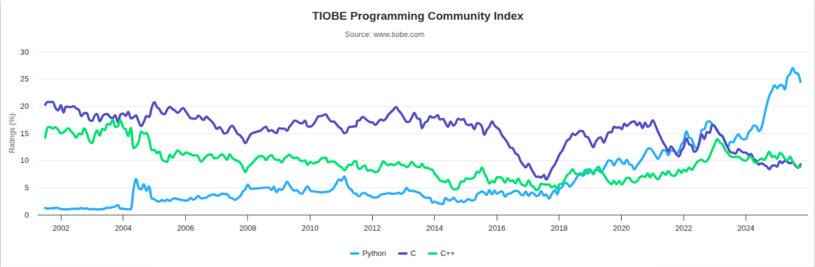
Over the years, the Python programming language has become increasingly popular in scientific computing, data analysis, and AI/ML, largely because of its expressiveness and it being widely supported by a broad community that enable rapid development. Although Python itself can be slow, much of the ecosystem achieves strong computational performance by relying on CPython bindings to optimized native libraries. Libraries like NumPy, SciPy, PyTorch and TensorFlow are prime examples of this: use Python for application logic, and leave optimized C/C++/CUDA kernels do the heavy lifting.
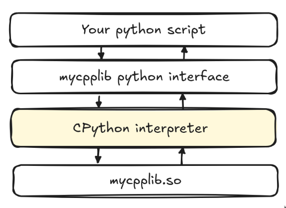
This Python as glue is great for productivity, but it can make performance debugging a bit unintuitive: a line of Python that looks cheap might just be a thin wrapper around a big C++ or CUDA operation. Therefore, profiling Python code concerns not only finding slow Python functions, but also about figuring out where the bottlenecks are – whether it is Python itself, bindings to native code, I/O, or kernels running on that accelerator (GPU/TPU) – and just timing the execution of the program. In practice, this means that there is no single profiler that fits every case: you usually start with a lightweight interpreter-level tool like cProfile to help you identify all the costly call paths, then zoom in with sampling profilers and system-level tools to probe even further. If your code makes use of accelerators like GPUs, you would then in turn have a look at the GPU timelines to see kernel launches, synchronization, and device utilization. With that in mind, we begin our quest for profiling our Python programs.
The optimization loop
It is important to not try to speculate about where performance bottlenecks in the code are, as doing so might lead to countless wasted hours. It is important to measure first before attempting to prematurely optimize the code. As the famous saying from a famous computer scientist and Turing Award winner, Donald Knuth goes:
“The real problem is that programmers have spent far too much time worrying about efficiency in the wrong places and at the wrong times; premature optimization is the root of all evil (or at least most of it) in programming”
And so you ought to adopt the following loop:
- Measure your program (using the right profiler)
- Identify the bottleneck based on profiler insights
- Optimize your code based on the profiler
- Repeat
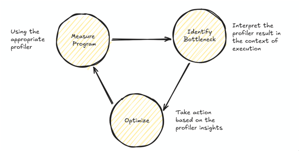
Essentially, this turns performance optimization into a search problem: the better the tools at displaying quick insights or the better your proficiency of the tools becomes, the tighter your optimization workflow can be and the faster you can iterate on your optimization goals.
Choose your profiling granularity
Choosing the right granularity for profiling is just as important as choosing the profiling tool itself, and it depends on which aspects of the program’s performance you already understand. You might have a clear picture of the algorithmic performance but not the architectural details (such as SIMD efficiency or GPU utilization) or you might not understand the program’s interaction with the OS, for example, how much time it spends in system calls, threads synchronization, or contending for shared resources. Profiling should be aimed at closing these gaps in your understanding.
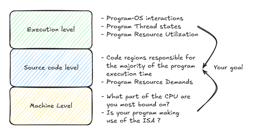
At each of these levels there exist a plethora of tools that allow you to collect information at the level you need, to locate identify the cause of the bottleneck(s) in your code. A few of them are below, but it is important to explore the different profilers to better accommodate your workflow and requirements.
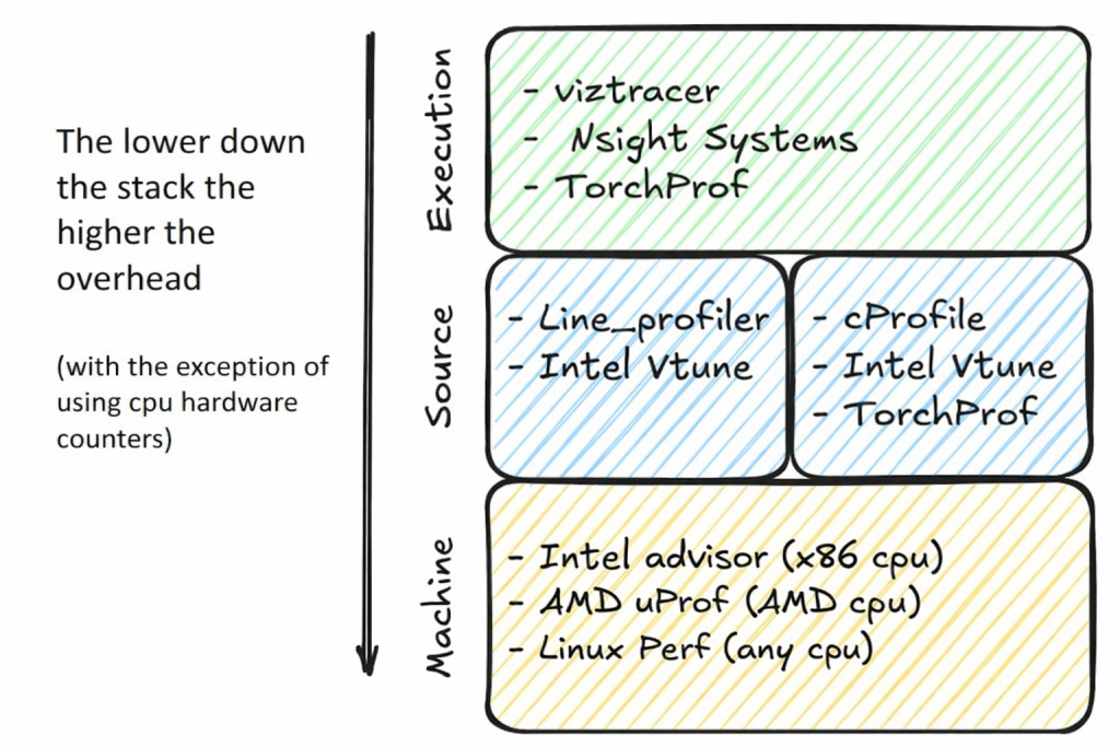
Profiling comes at a computational cost. Simply observing the program introduces overheads that can significantly slow down its execution, distorting its normal behavior and consume additional system resources such as memory and CPU cycles to collect, store, and analyze performance dat
Profiling hygiene checklist
- Ensure Accuracy
- Minimize measurement overhead which could be due to cold starts
- Account for outliers by running repeating benchmarks and averaging the runtimes
- Run for an adequate simulation length
- Ensure that your profiled program resembles the behavior of the real program
- Ensure Consistency
- Take fixed random seeds if you are generating the profiling data at each run of the profiler
- Set CPU affinity appropriate to the NUMA regions
- Run multiple times, with sufficient warmup
- Reduce measurement noise
- Run exclusively in the node(s) you allocate (passing
--exclusiveto Slurm) - If you time a kernel, time only that unless your goal is to understand the overall behavior of your application
- If you are running multi-node, try to allocated nodes as close as possible, such as in one rack
- Lock your GPU clock(s) if the system allows you to do so
- Check for CPU throttling
- Ensure consistent compilation using the same compiler version and compiler flags between runs
JUBE
JUBE (the Jülich Benchmarking Environment) is a lightweight, script-based framework that lets you define a benchmarking / workflow experiment, execute it and then evaluate the results in a structured way. JUBE becomes useful the moment you have two versions of the same program and you want to compare them: same machine, same arguments, same environment and just want to compare the impact of a set of code changes.
my_bench/
  compare.yaml
  baseline/train.py
  optimized/train.py
# baseline/train.py
import argparse, time, torch

def step(m,x,y,opt):
    opt.zero_grad()
    loss=0.0
    for i in range(x.size(0)):  # slow: per-sample Python loop
        loss += (m(x[i]).sub(y[i]).pow(2).mean())
    loss = loss / x.size(0)
    loss.backward(); opt.step()

def main():
    ap=argparse.ArgumentParser()
    ap.add_argument("--d",type=int,default=1024)
    ap.add_argument("--bs",type=int,default=128)
    ap.add_argument("--iters",type=int,default=200)
    args=ap.parse_args()

    dev="cuda" if torch.cuda.is_available() else "cpu"
    torch.manual_seed(0)
    m=torch.nn.Linear(args.d,args.d,bias=False).to(dev).train()
    opt=torch.optim.SGD(m.parameters(),lr=1e-3)
    x=torch.randn(args.bs,args.d,device=dev); y=torch.randn(args.bs,args.d,device=dev)

    step(m,x,y,opt)  # warmup
    t0=time.perf_counter()
    for _ in range(args.iters): step(m,x,y,opt)
    t1=time.perf_counter()
    print(f"ITER_MS: {(t1-t0)/args.iters*1e3:.3f}")

if __name__=="__main__": main()
# optimized/train.py
import argparse, time, torch

def step(m,x,y,opt):
    opt.zero_grad()
    (m(x).sub(y).pow(2).mean()).backward()  # fast: vectorized batch
    opt.step()

def main():
    ap=argparse.ArgumentParser()
    ap.add_argument("--d",type=int,default=1024)
    ap.add_argument("--bs",type=int,default=128)
    ap.add_argument("--iters",type=int,default=200)
    args=ap.parse_args()

    dev="cuda" if torch.cuda.is_available() else "cpu"
    torch.manual_seed(0)
    m=torch.nn.Linear(args.d,args.d,bias=False).to(dev).train()
    opt=torch.optim.SGD(m.parameters(),lr=1e-3)
    x=torch.randn(args.bs,args.d,device=dev); y=torch.randn(args.bs,args.d,device=dev)

    step(m,x,y,opt)  # warmup
    t0=time.perf_counter()
    for _ in range(args.iters): step(m,x,y,opt)
    t1=time.perf_counter()
    print(f"ITER_MS: {(t1-t0)/args.iters*1e3:.3f}")

if __name__=="__main__":
    main()
Conceptually, this benchmark sweeps over a variant parameter (baseline vs optimized), runs the same command for each, parses a timing metric from stdout, and produces a small results table:
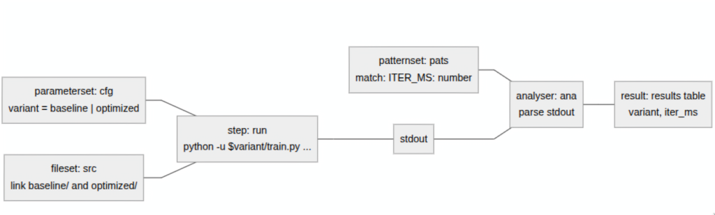
Here’s the complete JUBE configuration that does exactly that:
name: compare_versions
outpath: bench_run
comment: Compare baseline vs optimized

parameterset: # Configuration
  name: cfg
  parameter: {name: variant, _: "baseline,optimized"}

fileset: # Make both folders visible inside each sandbox
  name: src
  link:
    - baseline
    - optimized
step: # Run exactly the same workload for both variants
  name: run
  use:
    - cfg
    - src
  do: python -u $variant/train.py --iters 5

patternset: # Parse the metric
  name: pats
  pattern: # regexp that matches the iteration time from our program ex: "ITER_MS: 78.683"
    - {name: iter_ms, type: float, _: "ITER_MS: $jube_pat_fp"}

analyser:
  name: ana
  use: pats
  analyse:
    step: run
    file: stdout

# Print a small table
result:
  use: ana
  table:
    name: results
    style: pretty
    sort: variant
    column:
      - variant
      - iter_ms
And here is how you would run it from start to completion:
$ jube run compare.yaml
$ jube analyse bench_run
$ jube result bench_run
And you should see output along these lines:
######################################################################
# benchmark: compare_versions
# id: 2
#
# Compare baseline vs optimized
######################################################################

Running workpackages (#=done, 0=wait, E=error):
############################################################ (  2/  2)

  | stepname | all | open | wait | error | done |
  |----------|-----|------|------|-------|------|
  |      run |   2 |    0 |    0 |     0 |    2 |

>>>> Benchmark information and further useful commands:
>>>>       id: 2
>>>>   handle: bench_run
>>>>      dir: bench_run/000002
>>>>  analyse: jube analyse bench_run --id 2
>>>>   result: jube result bench_run --id 2
>>>>     info: jube info bench_run --id 2
>>>>      log: jube log bench_run --id 2
######################################################################
######################################################################
# Analyse benchmark "compare_versions" id: 2
######################################################################
>>> Start analyse
>>> Analyse finished
>>> Analyse data storage: bench_run/000002/analyse.xml
######################################################################
results:
|   variant | iter_ms |
|-----------|---------|
|  baseline |  25.683 |
| optimized |   1.984 |
Reasoning about your application's performance
“All models are wrong, but some are useful”
by George E. P. Box
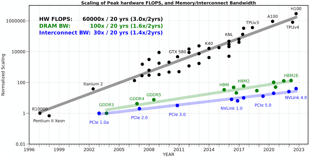
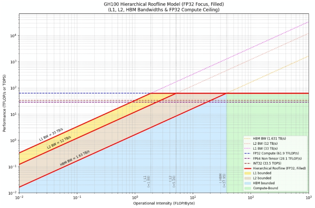
Over the years the gap between how fast we can compute and how fast we can move data has widened dramatically. As the figure below suggests, peak hardware FLOPs have increased orders of magnitude faster than DRAM/Interconnect bandwidth. The practical consequence is the well-known memory wall: for a growing fraction of real workloads, the limiting factor is not the amount of compute, but getting the right bytes to the right place at the right time.
This is also why latency-hiding mechanisms (caches, prefetchers, overlap of compute and communication, etc.) matter so much in practice: when you can successfully keep the data pipeline full, you can recover a surprising amount of otherwise lost performance. Using this insight, we can come up with a simplified first-order model of a kernel that helps identify the dominant bottleneck:
This naturally leads to the Roofline model idea: the performance you can achieve is bounded by either compute throughput or bandwidth, depending on your arithmetic intensity:
Concretely, you can end up classifying parts of your application as one of two regions:
- Compute limited your kernel is capped by peak FLOPs/s; the processor is busy doing arithmetic/logic operations,
- Bandwidth limited your kernel is capped by memory/interconnect BW; the processor frequently stalls waiting for data to arrive from cache/RAM.
A low arithmetic intensity implies the kernel is likely memory/communication-bound, while a high arithmetic intensity implies it is likely compute-bound.
For compute-intensive applications (machine learning, numerical simulation, etc.), this interplay between compute throughput and data movement is particularly critical. Knowing which side of the roofline you’re hitting guides optimization in very different directions: either you work to increase arithmetic intensity / reuse (so you move fewer bytes per FLOP), or you work to extract more bandwidth / hide latency (so you can feed the compute).
The roofline model – developed by Samuel Williams, Andrew Waterman, and David Patterson at UC Berkeley – visualizes exactly this tradeoff by plotting achievable performance versus operational (arithmetic) intensity. It makes the two fundamental ceilings explicit: peak computational throughput (peak FLOPs) and the bandwidth limit set by the memory system/interconnect. Below is a roofline graph for an Nvidia H100 GPU. In order to be compute bound your kernel or application would require an arithmetic intensity of at least 38 FLOPS/Byte to saturate the compute units.
Tools of the Trade
We are going to get acquainted with a few well known profilers that can be used to be used together in your quest of optimizing our Python programs, each providing a different perspective on our program.
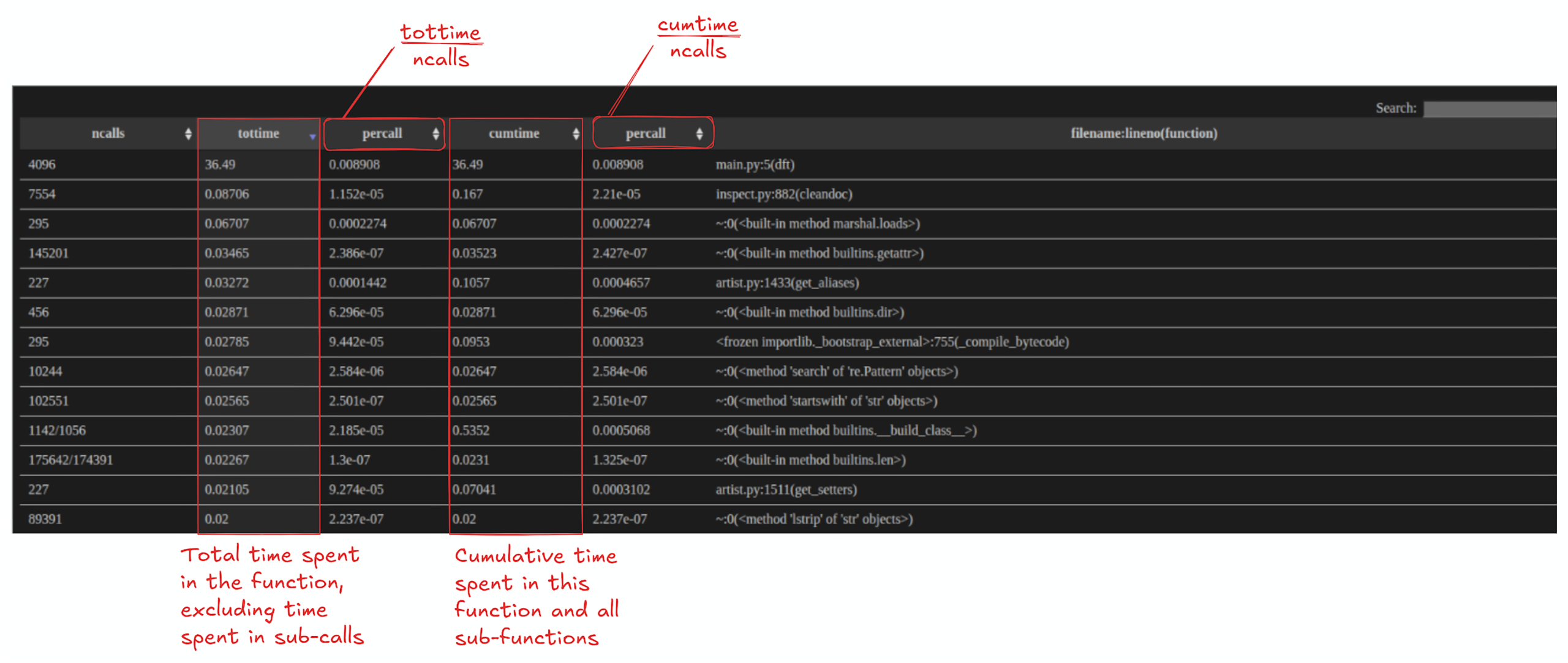
Tool 1: Start with cProfile
cProfile is used for function-level performance profiling in Python, mainly because it gives you a clear breakdown of where your program spends its time. It records how long each function takes (including cumulative time across calls) and how often functions are called, which makes it easy to identify hot functions that dominate runtime. This helps you quickly narrow optimization work to the few parts of the codebase that will deliver the biggest speedups, instead of guessing or micro-optimizing low-impact sections.
Since cProfile comes natively with Python you do not need to install anything:
$ python -m cProfile -o out.prof your_script.py
$ python -m cProfile -o <output-trace-name>.prof <your-py-script>.py
You can also profile regions of your program
import cProfile

pr = cProfile.Profile()
pr.enable()
main()
pr.disable()
pr.dump_stats("profile_output.prof")
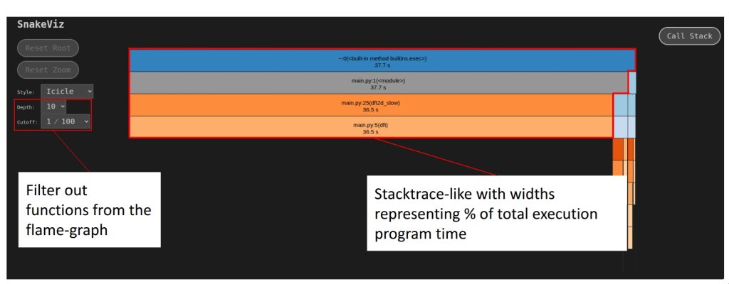
To view the generated profile statistics you can do so using snakeviz. But first you have to install it as follows:
$ pip install snakeviz
Once installed, you can visualize the generated cProfile output as such:
$ python -m snakeviz program.prof
Visualize with GraphViz
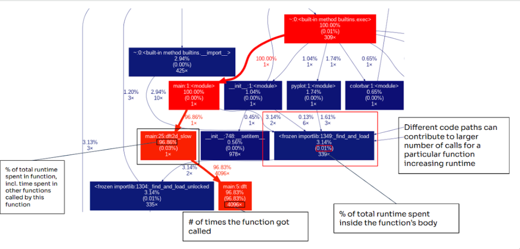
GraphViz is used in code optimization workflows because it supports the systematic visualization of program structure in forms that are directly relevant to performance. A GraphViz diagram can help you see the critical path of your application by showing you which functions call each other and the how much time you spend in each function.
To generate the diagram, first install gprof2dot, which converts your Python profiler output into a DOT graph that you can then render as an image.
$ pip install gprof2dot
To run gprof2dot using the default options you can run it as follows:
$ gprof2dot -f pstats <your-prof-file>.prof | dot -Tpng -o ./<prof-img>.png
This will generate a basic call graph from your profiling output and render it as a PNG. The diagram provides a quick way to spot which functions dominate runtime and how execution flows through your program. gprof2dot provides more options to add more profiling statistics to the graph, a few of which are below but you can checkout more in the gprof2dot’s Repository .
$ gprof2dot -f pstats --node-label=total-time --node-label=total-time-percentage --node-label=self-time-percentage <your-prof-file>.prof | dot -Tpng -o ./<prof-img>.png
Interpreting Graphviz
Once you generate the diagram, scan through the graph to identify the hotspots. Each node in the graph is a function or module, and each arrow shows a caller to callee relationship, so you can trace the execution flow from your entry point (often main or <module>) down into the functions it triggers. A quick way to determine the hotpath is to look at the colors of nodes. In general, warmer colors (reds) indicate functions that contribute more to overall runtime while cooler colors (blues) indicate functions with a smaller runtime impact to the total runtime of the program. If a node is bright red, it’s usually on the critical path or accounts for a large portion of total time of the program execution. If it’s dark blue, it is typically less important from a performance standpoint. The values in a node typically include:
- inclusive/total time (time spent in that function plus anything it calls)
- self time (time spent only inside that function’s own body),
- the call count (how often it was invoked)
This makes it easy to identify functions that are slow wherein most of the execution time is spent inside the functions body (high self time) versus functions that are expensive mainly because call other costly calls (high total time but low self time). In addition, some nodes may appear to be expensive not because each call is slow, but rather because they are invoked often.
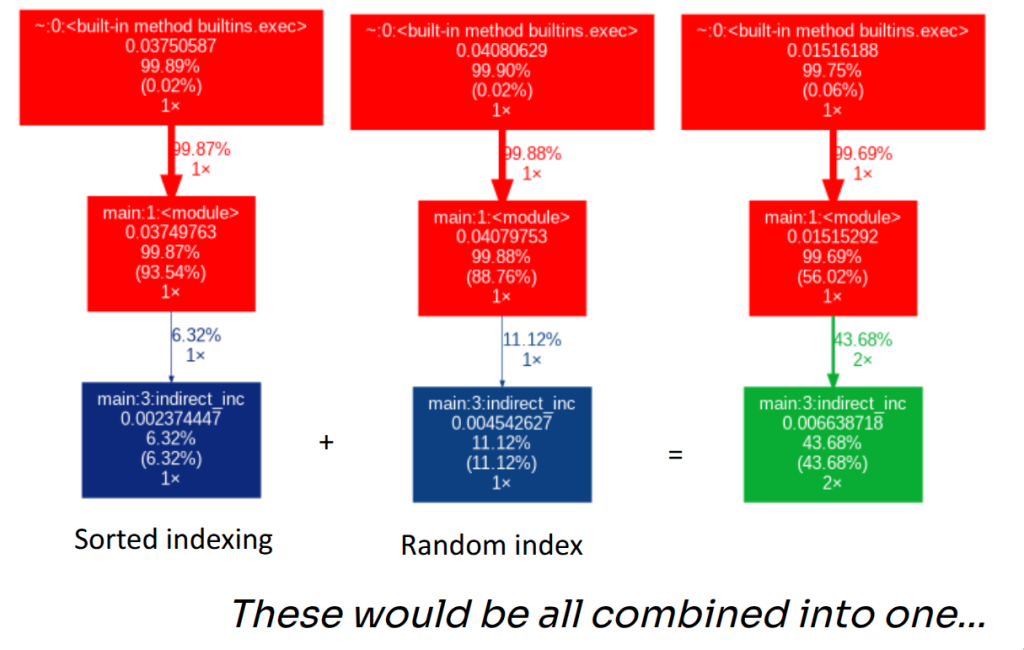
Problems with Graphviz
One of the down sides of using Graphviz is that nodes hold summary statistics, wherein different execution times of the same function from different calls paths of the program get aggregated into a single value.
N = 1 << 23
def indirect_inc(arr, index):
    for i in index: arr[i] += 1

arr = [0]* N

index = [i for i in range(N)]
indirect_inc(arr, index)

random.shuffle(index)
indirect_inc(arr, index)
In the above toy example, indirect_inc is called twice in our program, but the work it ends up doing on the CPU is completely different. The first call walks index that is in sorted order, so writes to arr proceed sequentially and play nicely with caches and prefetching. The second call writes through shuffled indices, turning the loop into essentially random memory writes, which creates far more cache misses and stalls.
If you profile these two calls separately, you get two very different pictures (fast sorted indexing vs slow random indexing). But when you run them in the same execution, Graphviz collapses both calls into a single indirect_inc node and reports one combined time. The result is the situation shown below: what were two meaningful distinct performance regimes get merged into one node, and the graph loses the information you actually care about – why the time is high and which invocation is responsible.
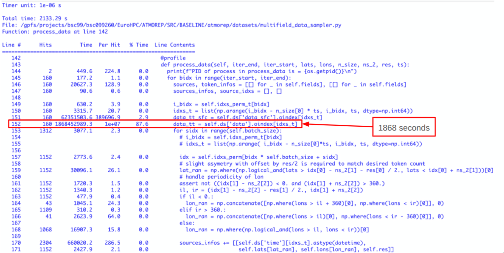
Tool 2: Use line_profiler when a single function is suspicious
line_profiler is used for line-by-line performance analysis, mainly because it lets you pinpoint the exact statements inside a slow function that are responsible for the runtime cost. While function profilers can tell you which function is slow, line_profiler shows why it’s slow by measuring time spent on each individual line (especially inside loops and heavy computations). That makes it ideal for targeted refactors as we will see later.
A classic example is chained indexing. It looks harmless, but it often performs multiple indexing steps and creates an intermediate array. Compare the two implementations below:
import numpy as np
n = 2**14
rows = np.random.choice(n, size=1000, replace=False)
cols = np.random.choice(n, size=1000, replace=False)
A = np.random.randn(n, n)
@profile
def bad_submatrix():
    return A[rows][:, cols]  # two indexing operations

@profile
def good_submatrix():
    return A[np.ix_(rows, cols)]  # one indexing operation

good_submatrix()
bad_submatrix()
bad_submatrix() does two separate indexing operations (and may allocate a temporary), while good_submatrix() uses np.ix_ to select the submatrix in a single operation.
To use line_profiler you will have to first install it, which you can simply do as follows:
$ pip install line_profiler
There are a couple of ways of using line_profiler . You can either use it to profile your whole application where you use it as such:
$ kernprof -l -v my_script.py
where
-lfor line-by-line profiling-vfor verbose output or without immediate output
and kernprof creates my_script.py.lprof.
Alternatively, you can inspect the created file without -v:
 $ kernprof -l my_script.py
 $ python -m line_profiler my_script.py.lprof
If you run line_profiler on the above script, you will usually see the extra cost show up immediately in the lines doing the indexing.
You can use line_profiler module to profile parts of your application by adding function decorators:
from line_profiler import profile

@profile
def slow_function(n):
    total = 0
    for i in range(n):
        for j in range(n):
            total += i * j
    return total

@profile
def another_function():
    result = []
    for i in range(1000):
        result.append(i ** 2)
    return result

if __name__ == "__main__":
    slow_function(1000)
    another_function()
which gives us the following profile result:
Timer unit: 1e-06 s

Total time: 0.633765 s
File: append.py
Function: slow_function at line 3

Line #      Hits         Time  Per Hit   % Time  Line Contents
==============================================================
     3                                           @profile
     4                                           def slow_function(n):
     5         1          0.7      0.7      0.0      total = 0
     6      1001        314.2      0.3      0.0      for i in range(n):
     7   1001000     307738.8      0.3     48.6          for j in range(n):
     8   1000000     325709.1      0.3     51.4              total += i * j
     9         1          1.9      1.9      0.0      return total

Total time: 0.000634606 s
File: test.py
Function: another_function at line 11

Line #      Hits         Time  Per Hit   % Time  Line Contents
==============================================================
    11                                           @profile
    12                                           def another_function():
    13         1          0.5      0.5      0.1      result = []
    14      1001        303.5      0.3     47.8      for i in range(1000):
    15      1000        330.0      0.3     52.0          result.append(i ** 2)
    16         1          0.6      0.6      0.1      return result
with the following column breakdown
| Column | Meaning |
|---|---|
| Line # | Source code line number |
| Hits | How many times this line was executed |
| Time | Total time spent on this line (in microseconds by default) |
| Per Hit | Average time per execution (Time ÷ Hits) |
| % Time | Percentage of total function time spent on this line |
Things to look for:
- High % Time on a single line (>50%)
- High Per Hit time (even with few hits)
- Unexpectedly high hits
- List comprehensions vs loops
Below is a real world example from a machine learning data processing step:
Tool 3: Timeline profilers when you care about GPUs, threads, or overlap
NVIDIA Nsight Systems is used for end-to-end performance analysis, mainly because it provides a system-wide view of how an application runs. It can help you visualize execution across CPUs and Nvidia only GPUs allowing you to spot where the majority of your application’s time is actually being spent and for what reason. Nsight thus allows us to focus our optimization efforts on the highest-impact bottlenecks.
$ nsys profile -t cuda,osrt,nvtx,cudnn,cublas -y 60 -d 20 -o <output_file_name> -f true <prog> <prog_args>
-t– Targets to be tracedcuda– GPU kernelosrt– OS runtime (e.g pread, pthread, etc)nvtx– NVIDIA Tools Extensioncudnn– CUDA Deep NN librarycublas– CUDA BLAS librarympi– Communicationpython-gil– Python’s Global Interpreter Lock contention and thread activity
-y– Delayed profile (sec)-d– Profiling duration (sec)-o– Output filename-f– Overwrite when it’s true<prog> <prog_args>– Execution command
You would use -y to skip the first stepts in the program, ideal for:
- JIT compilation (Torch Compile), CUDA context creation,
- Memory Allocation – for example OpenACC allocations at the start of the program,
and -d to capture “a subset of your program”:
- Say you want to capture a few iterations of a “solver”.
For more options you can read the NVIDIA Nsight Systems documentation, but the previous options are sufficient for most applications.
Once you have profiled your application, you can view the trace inside NVIDIA Nsight Systems, where it shows a complete visual view of the performance of your application.
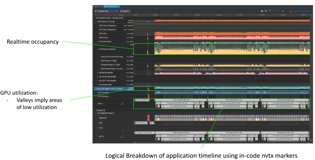
Generally you look at your nsys trace as two parts:
- Your Application view: Logical work that your application is doing
- Your Device/CPU view: What actually executing on the device/cpu
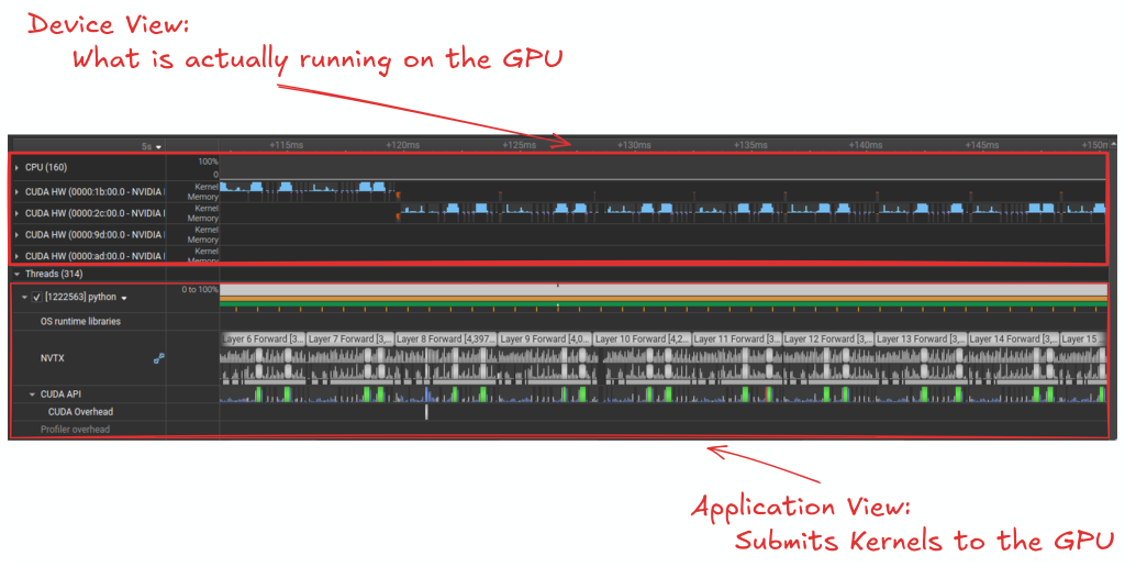
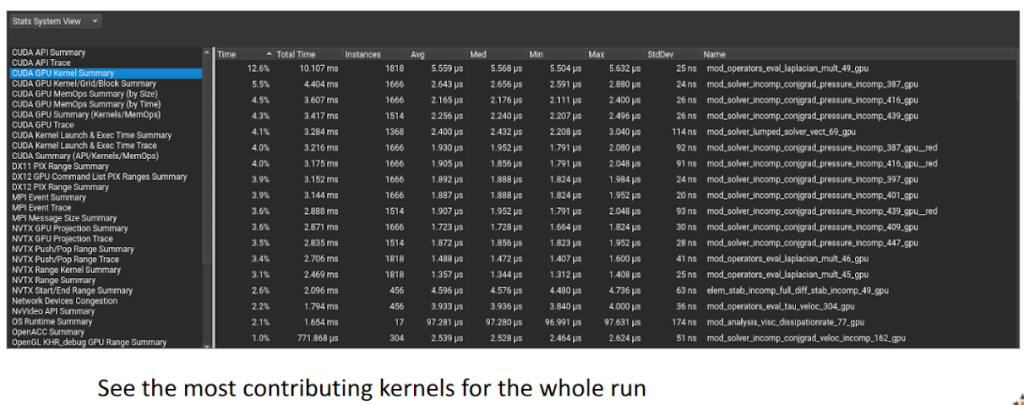
You are then able to dig deep into the runtime behavior of your application, looking at kernels that dominate the runtime of your application:
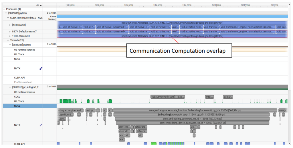
and look at your application with regards to how good your overlapping computation with communication.
Below we take a look at a few select examples of where Nsight systems might be useful in your optimization workflow.
Example: Python Global inerpreter lock (GIL)
Here we show an example of how Nsight Systems can show you the GIL behavior. In the example we perform an elementwise vector multiplication between two arrays a and b, and store the result into c. We split the work across multiple Python threads and wrap each worker in an NVTX range so that it shows up clearly in the nsys timeline.
from threading import Thread
import numpy as np
import time
import nvtx

N = 1 << 27
N_THREADS = 4

colors = ["blue", "green", "red", "yellow", "purple", "orange", "cyan", "magenta"]
def dot(a, b, c, lbl, color):
    with nvtx.annotate(f'dot {lbl}', color=color):
        for i in range(len(a)):
            c[i] = a[i] * b[i]

a = np.random.randint(0, 10, N)
b = np.random.randint(0, 10, N)
c = np.zeros_like(a)

chunk_size = N // N_THREADS
threads = []
start = time.time()
for i in range(N_THREADS):
    start_idx = i * chunk_size
    end_idx = (i + 1) * chunk_size if i < N_THREADS - 1 else N
    color = colors[i % len(colors)]
    t = Thread(target=dot, args=(
        a[start_idx:end_idx],
        b[start_idx:end_idx],
        c[start_idx:end_idx],
        str(i + 1),
        color
    ))
    threads.append(t)
    t.start()
for t in threads: t.join()
end = time.time()
print(f'Time: {end - start:.2f}')
To profile the application using Nsight System we do so as such:
$ export PYTHON_GIL=1 nsys profile --trace=nvtx,osrt,python-gil python ./main.py
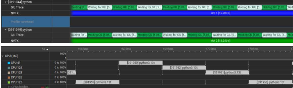
What we notice in the trace: In the GIL Trace lane, threads alternate between Holding GIL and Waiting for GIL. Looking at the CPU lanes, even though multiple threads exist, only one is making forward progress at a time on the Python loop because the work is dominated by Python bytecode due the the GIL.
Example: Python without GIL
We use the same code, but now we run a free-threaded Python build with the GIL disabled at runtime (the experimental PYTHON_GIL=0 mode). The workload is still memory-heavy, so you should not expect perfect scaling, but the structure of the execution changes immediately.
$ export PYTHON_GIL=0 nsys profile --trace=nvtx,osrt,python-gil python ./main.py
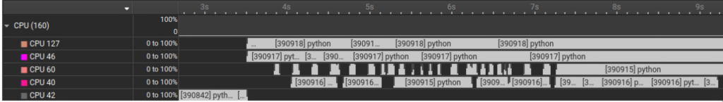
What we notice in the above trace is that CPU work is no longer serialized and we can clearly see a true overlap between the different running on multiple cores at the same time.
Example: Numba Cuda
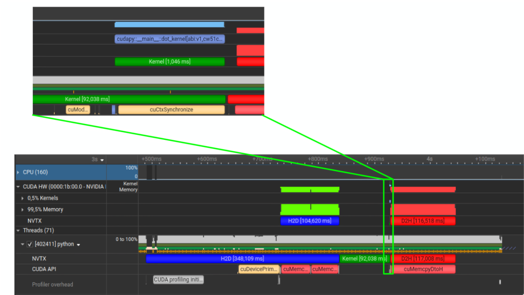
Here we use NVTX ranges to bracket the different phases of our simple CUDA program: H2D transfer, kernel, and D2H transfer. In real applications, you often bracket multiple kernels together that correspond to a logical step in your application. Doing so would allow you to focus on the logical parts of your application you can think of optimizing before directly jumping into optimizing separate kernels.
import numba
from numba import cuda
import numpy as np
import nvtx

N = 1 << 27

@cuda.jit(cache = True)
def dot_kernel(a, b, c):
    idx = cuda.grid(1)
    if idx < c.shape[0]:
        c[idx] = a[idx] * b[idx]

a = np.random.randint(0, 10, N, dtype=np.int32)
b = np.random.randint(0, 10, N, dtype=np.int32)

with nvtx.annotate('H2D', color='blue'):
    d_a, d_b = cuda.to_device(a), cuda.to_device(b)
    d_c = cuda.device_array(N, dtype=np.int32)

blocks = (N + 255) // 256
with nvtx.annotate('Kernel', color='green'):
    dot_kernel[blocks, 256](d_a, d_b, d_c)
    cuda.synchronize()

with nvtx.annotate('D2H', color='red'):
    result = d_c.copy_to_host()
$ nsys profile --trace=nvtx,osrt,cuda python ./main.py
Looking at the trace you can clearly see the following:
- The blue H2D block is the host to device copies (
cuda.to_device). - The green Kernel block is your GPU kernel execution.
- The red D2H block is device to host, which (in this example) is triggered by a synchronous
cudaMemcpyDtoH. - The moment you see
cuCtxSynchronize/cuda.synchronize()on the CUDA API lane, you have found a hard sync point. While not necessarily “bad” it often explains why transfers and kernels are not overlapping, since it effectively forces serialization. If you’re looking for overlapping execution, the timeline will usually tell you which exact API call is preventing this (a sync, an implicit sync copy, …)
Programmatic interface to nsys Profilers are measurement tools: they collect performance data about program we intend to profile and highlight what their authors believe is most important. That’s useful, but it also means the default views make certain assumptions about the most common workflows that the tool was designed for. The real benefit comes from treating the profiler as something you can bend to your needs allowing you to choose the metrics that matter for your hypotheses, as well as filtering and aggregating results for comparison across runs. The defaults get you started, but the tool becomes far more valuable once you shape it to your questions.
Nsight Systems can export traces into a SQLite database, which is really useful if you want to automate comparisons ex. CI performance checks or Checking for ” how much did this code change slow down kernels in my program?”. A common workflow is:
# 1) Capture
$ nsys profile -o report --trace=cuda,nvtx,osrt python ./main.py

# 2) Export to sqlite (creates report.sqlite)
$ nsys export --type sqlite -o report.sqlite report.qdrep
Then you can query kernel timings:
def extract_kernel_timings(db_path: Path) -> pd.DataFrame:
    """Extract kernel timings from SQLite database"""
    # Flatten kernel pairs to get a list of all kernel names
    valid_kernels = [kernel for pair in kernel_pairs for kernel in pair]

    with sqlite3.connect(f"file:{db_path}?mode=ro", uri=True) as conn:
        if not table_exists(conn, "CUPTI_ACTIVITY_KIND_KERNEL"):
            return None

        query = """
        SELECT s.value AS kernel_name,
               k.start,
               k.end,
               (k.end - k.start) AS duration_ns
        FROM CUPTI_ACTIVITY_KIND_KERNEL AS k
        JOIN StringIds AS s ON k.demangledName = s.id
        """

        df = pd.read_sql_query(query, conn)
        # Only keep rows where kernel name is one of the valid ones
        df = df[df['kernel_name'].isin(valid_kernels)]
        if df.empty:
            return None

        # Convert nanoseconds to milliseconds
        df['duration_ms'] = df['duration_ns'] / 1e3
        return df

except sqlite3.DatabaseError as e:
    print(f"Error reading {db_path.name}: {str(e)}")
    return None
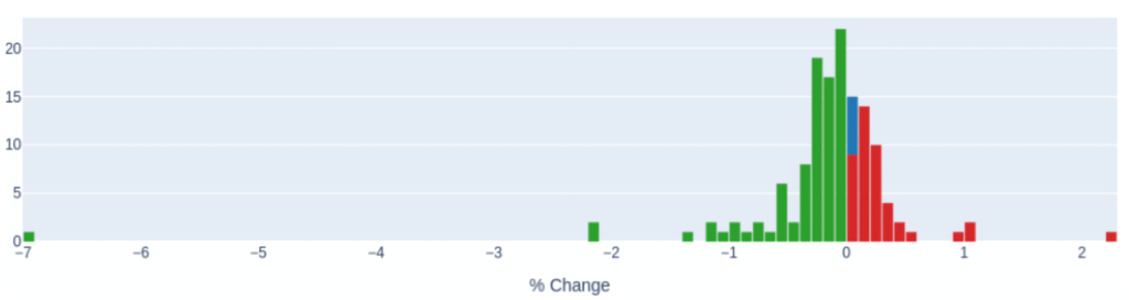
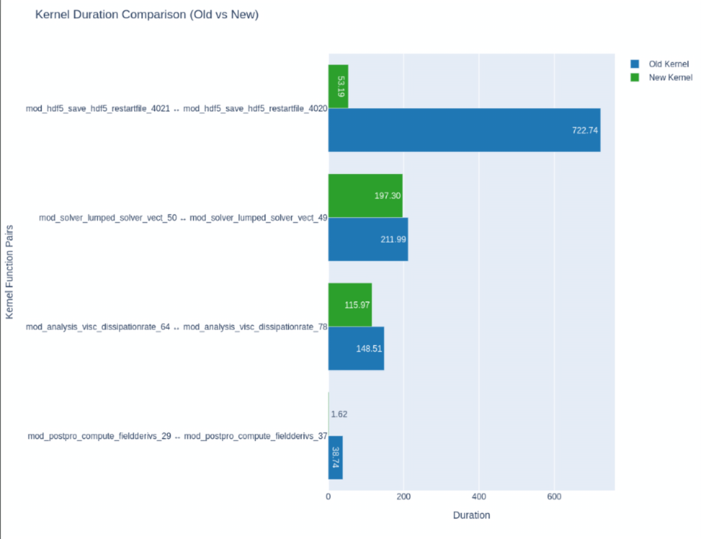
These can be helpful if you want to compare between multiple traces. Here below we compare the runtimes of all the kernels inside a particular program after a minor change. (Admittedly the traces are from a Fortran program but you can just as well do the same with your Python traces )
Or you can try to visualize the Speed-Of-Light (SOL) of a subset of kernels of your applications — Speed-Of-Light (SOL) is the percentage of theoretical peak performance/throughput per SM (Streaming Multiprocessor) / memory subsystem.
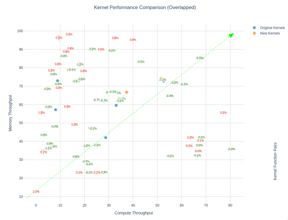
After which you optimize them, then compare between baseline and optimized versions:
You can read more about the NSYS’s SQLite schema here or learn how to use NVIDIA’s provided recipes, or even create your own by using NVIDIA’s recipes as templates.
Closing Remarks
To summarize, if your goal is to optimize Python code, a reliable workflow is:
- Measure end-to-end wall time (baseline).
- Use
cProfile(or sampling) to find hottest call paths. - If the hot path is Python: use
line_profiler. - If the hot path is native/GPU: use a timeline profiler (NVIDIA Nsight Systems / XProf).
- Turn the best hypothesis into a benchmark (JUBE / pytest-benchmark / similar).
- Repeat.
What matters most is not the specific profiler, but the idea of tightening the loop between observation and change. Start with coarse measurements that preserve context (overall wall time and call paths), then increase resolution only where evidence indicates it is warranted. This reduces the risk of optimizing the wrong thing and keeps profiling overhead proportional to the insight you are trying to obtain.
When accelerators are involved, be particularly cautious about attribution. Various Python APIs enqueue work asynchronously, apparent Python time can simply be launch overhead, while the real cost appears later as synchronization or idle gaps in the device timeline. In such cases, the timeline view is often the fastest way to establish whether you are compute-bound, bandwidth-bound, or simply under-utilizing the device due to serialization and host-side stalls. NVTX annotations are a practical way to reconnect timeline regions to application-level intent, which is essential once traces become non-trivial.
Finally, treat every optimization claim as a hypothesis until it survives a benchmark that is representative, repeatable, and appropriately controlled. The purpose of tooling such as JUBE or pytest-benchmark is not merely convenience, but to make performance changes auditable and comparable over time.
More code and samples can be found in the following repository.
References
- Python Software Foundation. The Python Profilers (profile, cProfile) (Python documentation). (Python documentation)
- Python Software Foundation. pstats — Statistics for profilers (Python documentation). (Python documentation)
- SnakeViz. SnakeViz documentation (cProfile visualization). (Jiffy Club)
- Fonseca, J. R. gprof2dot: Converts profiling output to a dot graph (GitHub repository). (GitHub)
- Graphviz. DOT Language documentation. (Graphviz)
- pyutils. line_profiler / kernprof documentation (ReadTheDocs). (Line Profiler)
- NumPy Developers. numpy.ix_ documentation. (NumPy)
- NVIDIA. Nsight Systems User Guide (documentation). (NVIDIA Docs)
- NVIDIA. NVTX annotation tool for profiling code in Python and C/C++ (developer blog). (NVIDIA Developer)
- Python Software Foundation. Python support for free threading (How-To;
PYTHON_GIL,-X gil). (Python documentation) - PEP 703. Make the Global Interpreter Lock Optional in CPython. (Python Enhancement Proposals (PEPs))
- Jülich Supercomputing Centre (FZJ). JUBE Benchmarking Environment (overview). (Forschungszentrum Jülich)
- Jülich Supercomputing Centre (FZJ). JUBE Documentation. (FZ Jülich Apps)
- Williams, S., Waterman, A., & Patterson, D. Roofline: An Insightful Visual Performance Model for Multicore Architectures (ACM). (ACM Digital Library)
- Wulf, W. A., & McKee, S. A. Hitting the Memory Wall: Implications of the Obvious (ACM). (ACM Digital Library)
- Knuth, D. E. Structured Programming with go to Statements (ACM, 1974). (ACM Digital Library)
- benfred. py-spy: Sampling profiler for Python programs (GitHub repository). (GitHub)
- pytest-benchmark. pytest-benchmark documentation. (pytest-benchmark)
- NVIDIA. Nsight Compute User Guide (kernel profiling documentation). (NVIDIA Docs)
- SAS (Rick Wicklin). On the source of “All models are wrong, but some are useful” (blog). (blogs.sas.com)
- Gholami, A., Yao, Z., Kim, S., Hooper, C., Mahoney, M. W., & Keutzer, K. AI and Memory Wall. arXiv:2403.14123 (2024).